
Can You See a Bearing Failure Coming? A Causal Monitoring Pipeline on the NASA/IMS Dataset
When I’m working on a bike and want to know whether a bearing is shot, I touch a wrench to the bearing housing and press the other end against the bone behind my ear. The wrench conducts the vibration straight to my skull, bypassing the air entirely — and what comes through is surprisingly clear. A good bearing barely registers: smooth rotation, almost silent. A worn one announces itself.
Unplanned mechanical failure is expensive. A bearing that fails mid-operation doesn’t just cost a replacement part — it costs downtime, collateral damage, and the kind of emergency that pushes maintenance teams into reactive mode. The interesting question is: can you see it coming in the data?
The NASA/IMS bearing dataset offers a controlled version of that question. Three experiments each ran a set of 4 roller bearings under constant load until one failed. Accelerometers sampled at 20 kHz, producing one 1-second file every 10 minutes — a timestamp-indexed stream of raw vibration. For Sets 2 and 3 (outer-race failures, the cleaner failure mode), the experiments ran roughly 7 days before the failure event.
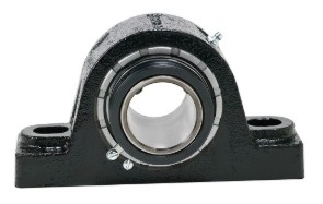
The Rexnord ZA-2115 double-row roller bearing
I built a pipeline to answer two questions: Does the degradation signal emerge from the noise early enough to be useful? And does a model trained on one experiment work on another it has never seen?
The constraint: causal-only processing
The easiest way to make a monitoring pipeline look good in hindsight is to use future data. A symmetric filter, for instance, smooths by averaging forward and backward in time — which means it “knows” what happens next. A real monitoring system doesn’t get that luxury.
Every step of this pipeline is strictly causal — outputs at time t depend only on data at or before t:
- Causal Gaussian smoothing via an FIR filter (
scipy.signal.lfilter). The kernel peaks at the current sample and decays into the past:h[k] = exp(-0.5·(k/σ)²)for k = 0, 1, …, W. This is the same smoothing a live dashboard would apply as new samples arrive. - Feature extraction is computed per file-snapshot from the smoothed signal — no look-ahead.
- PCA normalization and projection for Set 3 use Set 2’s statistics. The model is frozen before Set 3 data is seen.
From raw signal to a degradation index
Four channels of smoothed vibration are aggregated per file into 16 statistical features: mean, RMS (root mean square), peak-to-peak range, and excess kurtosis for each channel. These capture amplitude, energy, spread, and impulsiveness — the four things that change as a bearing degrades.
PCA reduces those 16 features to 3 principal components. The first component (PC1) explains the dominant variance in the feature space. In a well-functioning bearing, that variance is noise. In a degrading one, it’s the failure signature.
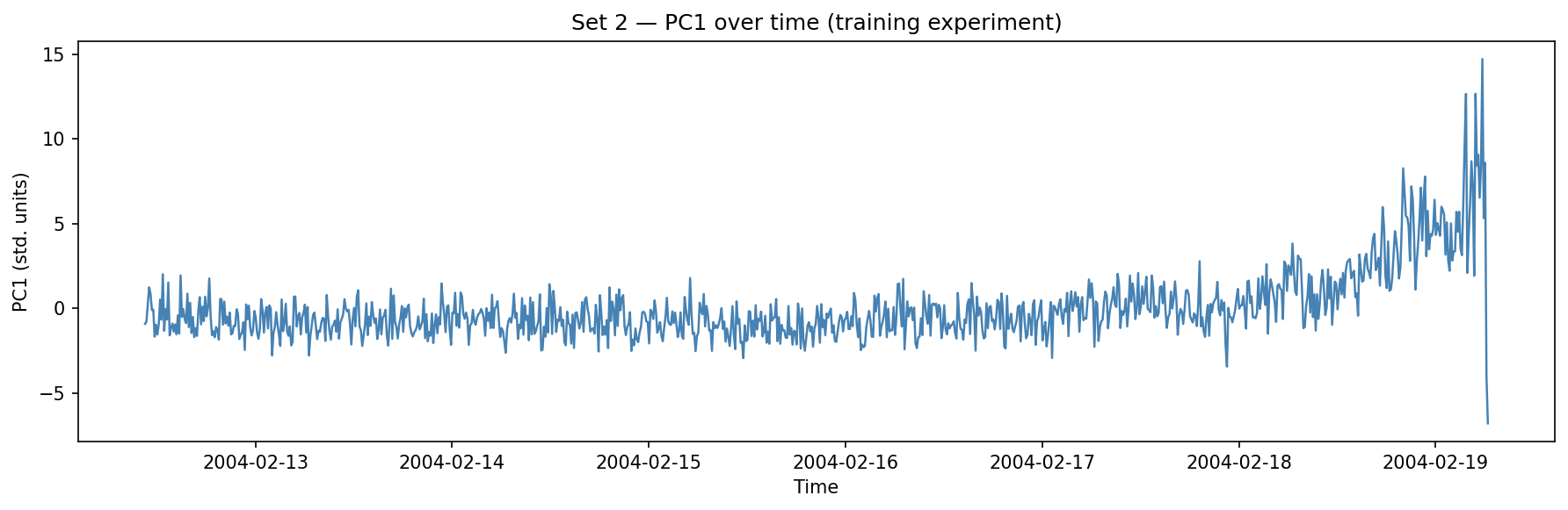
Set 2: PC1 trends monotonically upward across the final two days of the experiment.
That upward trend is the degradation signal. It’s not a single spike — it’s a gradual, accelerating drift that the pipeline can track in real time.
Derivatives as an early warning signal
Changepoint detection finds when PC1 shifts between stable regimes. That’s useful for segmenting the timeline, but it conflates “the bearing settled into a new operating state” with “the bearing is actively failing.” The two look identical to a changepoint detector.
Each derivative is smoothed with a rolling mean (30-snapshot window) to reduce noise from the numerical gradient.
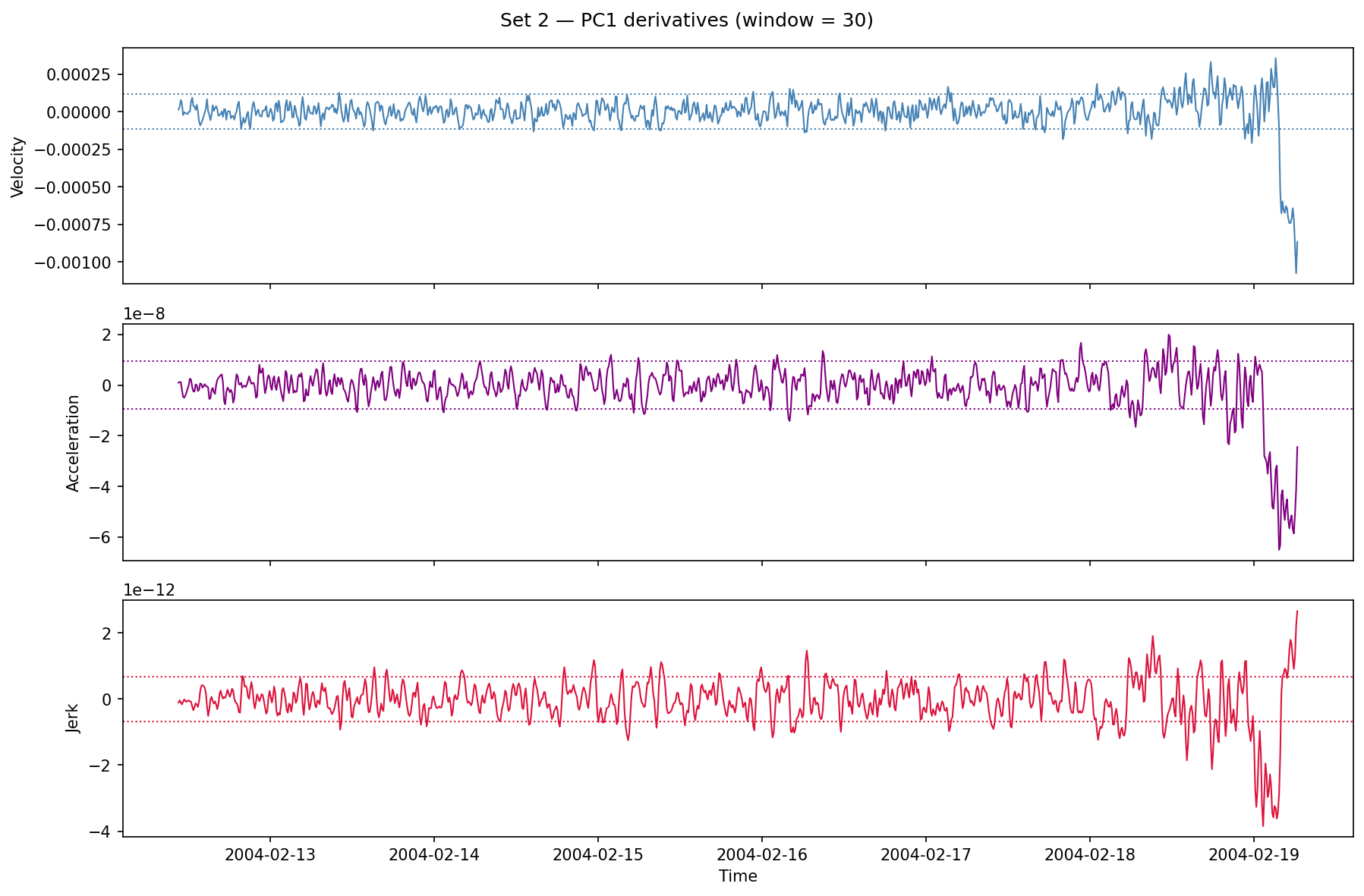
Velocity, acceleration, and jerk of Set 2 PC1. The dotted lines are ±1 STD computed over the full experiment. Sustained exceedance of those bands — particularly in acceleration — is the candidate alarm.
The pattern is consistent with what you’d expect from progressive mechanical damage: a long flat period, followed by a period of rising velocity, followed by a sharp acceleration spike as the failure event approaches.
Blind evaluation on Set 3
Set 3 is a different bearing, a different experiment, and a different failure event. The pipeline is applied identically — same KERNEL, same LOOKBACK, same N — but the normalization parameters (mean and standard deviation) and the PCA eigenvectors are the ones computed on Set 2. Set 3 data is never used to fit anything.
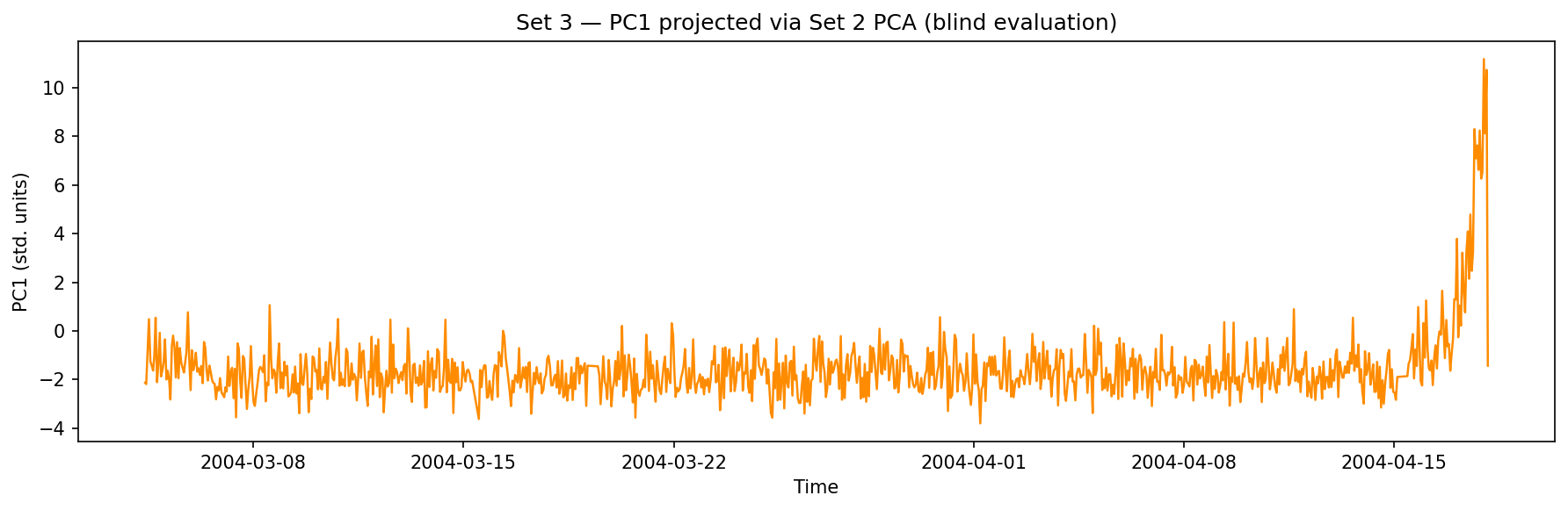
Set 3 PC1, projected through Set 2’s frozen model. The degradation trend is visible under the same signal processing.
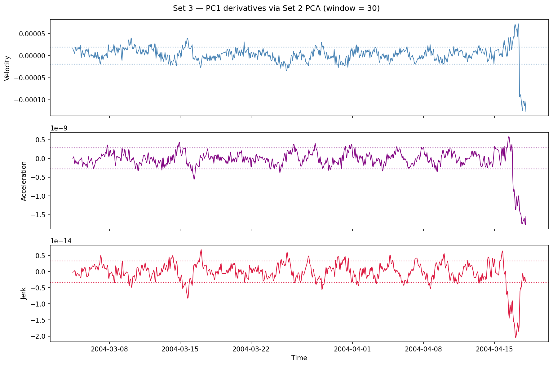
Set 3 PC1 derivatives. The same velocity/acceleration spike pattern emerges near the end of the experiment.
The degradation signal generalizes. The model learned something about outer-race failure dynamics in Set 2, and that representation is meaningful in Set 3 — even though the two experiments used different bearings with different initial conditions and ran for different lengths of time.
What this means in practice
The core idea here is condition-based maintenance: instead of replacing bearings on a fixed schedule or waiting for failure, you monitor the signal and act when the degradation index crosses a threshold. That threshold can be set on the derivatives — sustained acceleration above 1 STD, for instance — rather than on the raw PC1 value, which means it’s sensitive to rate of change rather than absolute level.
This kind of pipeline is particularly useful when:
- Failure mode is consistent (outer-race failure here; a different mode would need revalidation)
- Training data is available from at least one controlled run
- A live monitoring system needs to process new experiments without retraining
Limitations. The published dataset doesn’t include ground-truth failure timestamps, so we can’t precisely quantify how much lead time the signal provides. Downsampling at N=500 (every 500th raw sample) trades temporal resolution for speed; a production system would process the full 20 kHz stream. Set 1 — a more complex multi-bearing, mixed-mode failure — is not analyzed here.